Side-Channel Trace Analyzer Tool

Description

Side-Channel Analyzer is a desktop application for analyzing side-channel traces of encryption algorithms. It is specifically designed for performing Differential Power Analysis on AES power traces. Other features may be added in the future.

Project Info

• Issue tracking: https://github.com/tmtemetm/side-channel-analyzer/issues
• External Dependencies:
  • JDK 11 or higher

Running

Make sure you have JDK 11 or higher installed on your machine. Oracle provides an installation guide for the latest java version (15) for Linux, macOS and Microsoft Windows at https://docs.oracle.com/en/java/javase/15/install/overview-jdk-installation.html. You can also use OpenJDK.

Download the jar file side-channel-analyzer-1.0.0-RELEASE.jar from https://github.com/tmtemetm/side-channel-analyzer/releases/tag/1.0.0-RELEASE.

If you have the JDK correctly set, the jar file should run by double-clicking. Otherwise, you can also run it from the command line with

java -jar side-channel-analyzer-1.0.0-RELEASE.jar

Local Development Setup

• Install OpenJDK 11 or higher
• Clone this Git repository

  git clone git@github.com:tmtemetm/side-channel-analyzer.git
  

• Build the package using either the provided maven wrappers or with a local maven installation:

On Unix:

./mvnw clean package

Or on Windows:

mvnw.cmd clean package

• Run the application with

  ./mvnw spring-boot:run
  

  or, if you prefer,

  java -jar target/side-channel-analyzer-1.0.0-RELEASE.jar
  

Operating Principle and Examples

Differential Power Analysis is a side-channel attack, which means that it makes use of information exchange with the cryptographic module that is not part of its intended function. It is based on the observation that the power consumption of a computing unit is dependent on the data it processes. The dependence can arise, for example, from power leakages of semiconductor chips during logic transitions.

In contrast to simple power analysis, differential power analysis measures the power consumption of a cryptographic module during multiple runs of the cryptographic operation and analyzes these power traces statistically. One way of statistically analyzing the power traces is to correlate the power traces at a specific time instant to a hypothesized power model.

Below, we go through the operating principle of the DPA implementation with an example measurement.

Measurement Setup and Trace Data

We use an example measurement of an externally powered chip performing 128-bit AES. The chip was connected to a computer that sent encryption instructions with randomly selected 128-bit plaintexts to the chip. The power consumption of the chip was measured with an oscilloscope.

Example measurement traces and plaintexts can be found at https://github.com/tmtemetm/side-channel-analyzer/releases/tag/1.0.0-RELEASE. The examples are located in the examples.zip file.

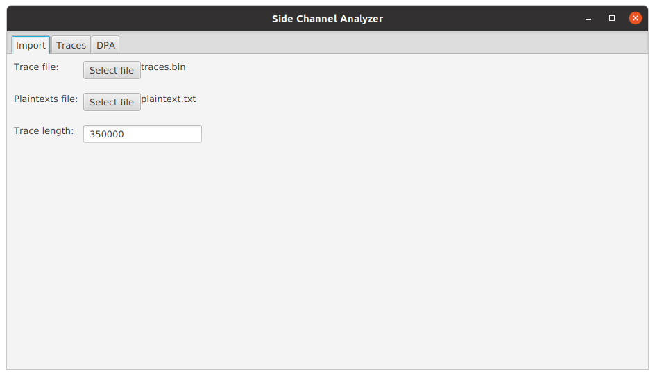
Importing Traces in Side-Channel Analyzer

The Side-Channel Analyzer tool currently expects the import file to contain the traces in binary format as 8-bit unsigned integers with no separators between the traces, though additional formats may be supported in the future. The tool also expects a file containing the plaintexts used for encryption with each plaintext on its own line and whitespace separating the individual bytes in hexadecimal. The trace length is primarily inferred from the length of the trace file and the number of plaintexts. If unsuccessful, it has to be input by the user.

Plotting Traces in Side-Channel Analyzer

After the traces and plaintexts have been imported, the user can plot the traces under the Traces tab. The figure figure shows the initial view of the traces tab.

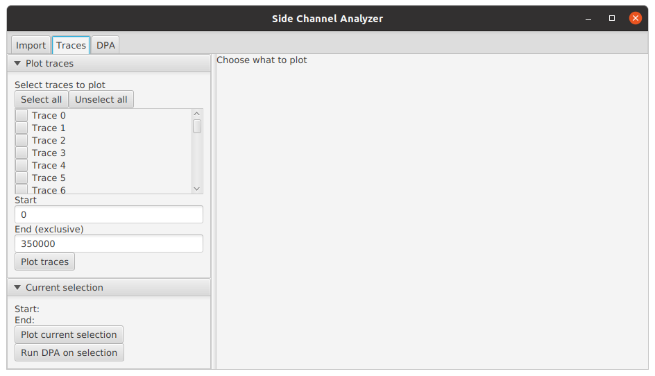
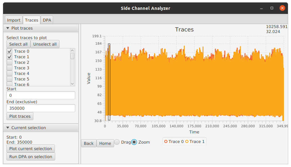
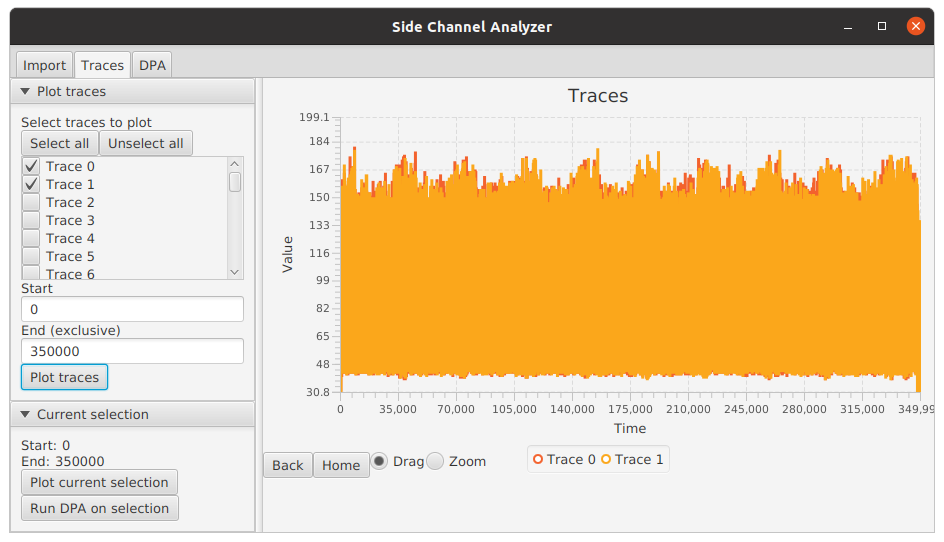
On the left, the user can select which traces to plot and the starting and ending points for plotting. As an example, the figure below shows the plot of the first two traces (Choose Trace 0 and Trace 1 and press Plot traces). We can immediately notice 10 bumps of larger power consumption, which correspond to the 10 rounds of 128-bit AES.

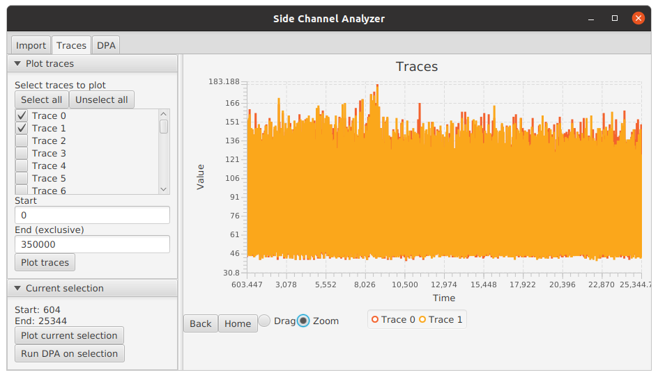
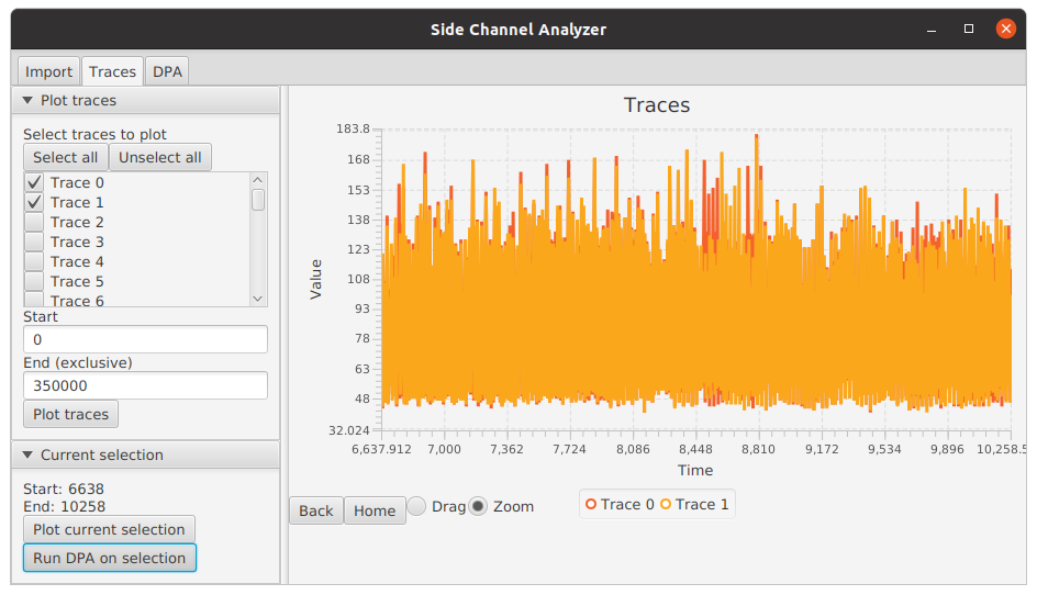
The traces can be examined using the drag and zoom functionalities by dragging over the image. The tool in use can be changed using the radio buttons below the plot area. The Back and Home buttons allow reverting to previous views or to the first view. Below we have zoomed over the first AES round.

Plotting a large amount of full traces is not recommended, since the full traces consume a lot of memory. If one wishes to view a large amount of traces at once, they should be plotted only within a small interval using the Start and End inputs.

Performing Differential Power Analysis

Differential power analysis can be started from the DPA tab. The user can input the number of traces to include in the analysis and the starting and ending points of the time interval to consider for the analysis. Alternatively, the user can set the interval to the currently plotted interval by pressing Run DPA on selection under the Traces tab. The interval should not be set too long (tens of thousands), since the analysis is quite computationally expensive.

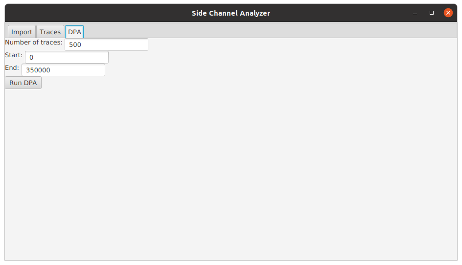
To perform the DPA, press Run DPA. This will open a new tab for inspecting the results. Let's see how's the analysis conducted.

Description of the Algorithm

As mentioned above, differential power analysis analyzes the power traces of multiple runs of a cryptographic operation statistically. The algorithm in Side-Chanel Analyzer uses a hypothesized power model and correlates it with the observed power consumptions across traces.

The Power Model

The algorithm targets the individual bytes in the output of the first SubBytes step. The step is preceded by the AddRoundKey step, where the plaintext is XOR-ed with the first round key. Then, the individual bytes are transformed with a so-called S-Box, which performs a non-linear transformation on the bytes.

The value after the first SubBytes is a good candidate for power analysis. Since the S-Box is often implemented as a look-up table, the value is read from memory and with some hardware implementations, the power consumption of reading from memory is largely dependent on the Hamming weight (number of set bits) of the returned value. Additionally, the operation following SubBytes is ShiftRows, which shifts the byte within the block but leaves the byte in tact before passing it to the next step, the MixColumns step.

The bytes after the first SubBytes operation are also easy to model, since they are only affected by a single byte of the round key. Each byte in the output of the SubBytes operation can be calculated by XOR-ing the corresponding byte of the plaintext with the corresponding byte of the round key and passing that value through the S-Box. This implies that the DPA can be performed on individual bytes separately, instead of having to consider the whole round key. Roughly, this means that the complexity of the analysis is reduced from 2¹²⁸ to 2⁸, although in practice it is not quite that simple.

Based on the above discussion, the Hamming weight of the output value of the first SubBytes operation is a good candidate for a power model. In practice, the algorithm

• considers each byte position in the round key separately,
• iterates through all the 2⁸ possible bytes for that position,
• XOR-s the key with the corresponding plaintext position,
• looks up the S-Box value for the XOR-ed value,
• hypothesizes the power consumption by computing the Hamming weight of the S-Box output, and
• correlates the hypothesized power consumptions with the measured ones across multiple traces.

The last phase is discussed in more detail in the next section. Other power models are also possible, but the Hamming weight of the first SubBytes output seems to work well in practice. Other power models may be added to Side-Channel Analyzer in the future.

Correlating the Hypothesized and Measured Power Consumptions

Suppose for now that we know the correct time instant t where the modeled value (e.g., the output of the first SubBytes step) is processed. The distribution of power consumptions at time t across traces should follow approximately the hypothesized power consumptions calculated using the power model and the currently considered byte position, if the key byte was correctly hypothesized. Of course there will be extra noise, notably from the remaining 15 byte positions that are not being considered.

On the other hand, if the hypothesized key byte is wrong, the hypothesized power consumptions should not correlate with the measured ones if the hypothesized key byte is wrong, since the power hypothesis (e.g., the hamming weight of the SubBytes output) will also be wrong. To find out the correct key byte, we can therefore iterate through all 2⁸ possible key bytes and correlate the hypothesized power consumptions with the measured ones at time t. The correct key byte should be the one with the highest correlation.

Since in reality, we don't know the correct time instant t, we'll also need to iterate through a time interval t₁,...,t_l, correlate all key-time pairs and choose the key byte and time instant with the highest correlation. For computing the correlations, we use the Pearson's correlation coefficient due to its simplicity.

The algorithm has to compute 2⁸l correlations for all byte positions, where l is the length of the time interval. Choosing a wider time interval increases the possibility of finding the correct time instant but increases the running time of the algorithm.

An Example in Side-Channel Analyzer

We will run an example DPA using the Side-Channel Analyzer tool. From the plot of the first two traces below, we can recognize the 10 rounds of a 128-bit AES.

We also notice a large spike in power consumption that is present in many of the other rounds as well. Hoping that the modeled intermediate value is processed somewhere around that spike, we zoom in around that spike.

We then send the currently shown interval to the DPA feature by pressing Run DPA on selection.

We leave the settings as they are and press Run DPA.

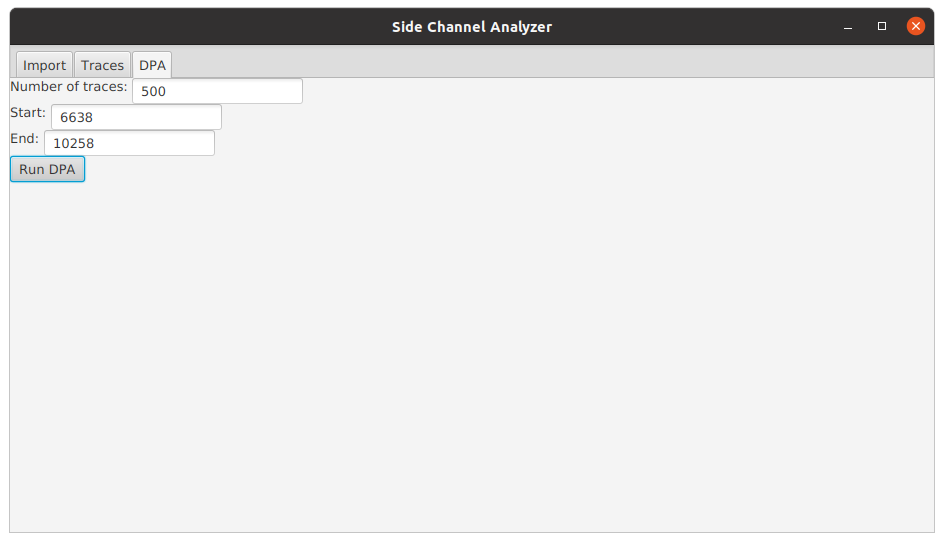
This will open a new tab with the results. The tool analyzes the bytes in parallel and updates the results as they finish.

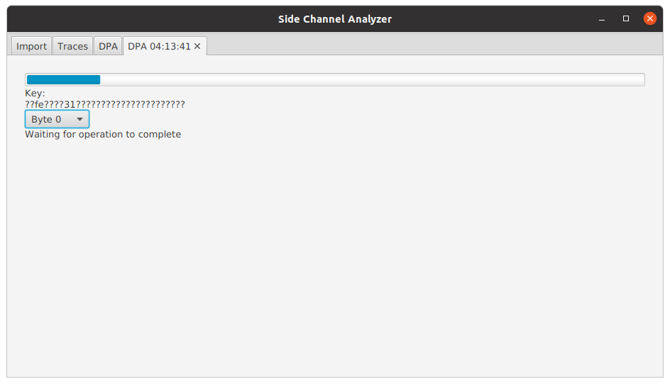
The key string presents the completed key bytes in hexadecimal and ?? for uncompleted bytes. The presented string is the round key, but conveniently for the first AddRoundKey operation of a 128-bit AES, the round key equals the encryption key.

Individual bytes can be examined by selecting the desired byte position from the choose box. The table lists the byte value hypotheses with the best result first. For each hypothesis, the table presents the time instant with the highest correlation, the correlation between the hypothesized and measured power consumptions at that instant, and an approximate p-value for the correlation.

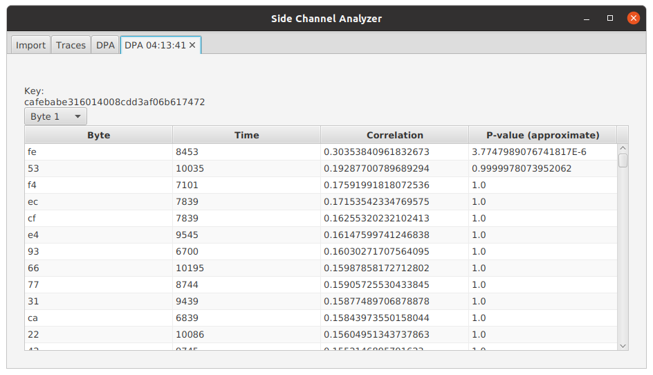
The p-value provides a good way for interpreting whether the found key byte is likely to be correct or not. The p-value tells the probability of obtaining the observed correlation if no correlation is assumed. A p-value of 0.05 therefore implies that there is a 5 % probability of making the wrong conclusion if we conclude that the hypothesized and measured power consumptions are correlated. Therefore, a p-value of 0.05 in the output of the algorithm tells us that there's a 5 % probability of picking the wrong key byte. The p-values output by the algorithm should be considered approximate, since the underlying assumptions behind the computation of the p-value are not necessarily fully met. Nevertheless, the p-values provide a good tool for approving or rejecting the output of the algorithm. The lower the p-value, the better the result.